Course map
Course structure
The chapters follow the nnsyn workflow. We begin with the MRI-to-CT task, then follow the data through planning, preprocessing, the network, training, inference, and evaluation.
- 01The taskWhy MRI → CT?
- 02What is nnsyn?Inheritance + changes
- 03Data & plansFiles → self-configuration
- 04ArchitectureContext + detail
- 05LossesWhat is optimized?
- 06TrainingUpdate → checkpoint
- 07InferencePatches → HU volume
- 08EvaluationNumbers + images
- 09Hands-onTrained validation run
- 10TakeawaysCheck understanding
01
Clinical task
Clinical motivation
Why synthesize CT from MRI?
MRI gives excellent soft-tissue contrast without ionizing radiation, but its voxel values depend on the scanner and acquisition sequence. CT has a calibrated numerical scale: Hounsfield units describe X-ray attenuation and support tasks such as radiotherapy dose calculation.
The practical goal is an MRI-only workflow that estimates the CT volume instead of acquiring a separate CT. The model predicts one CT value at every MRI voxel, so the two volumes remain spatially aligned.
→
nnsyn
3D translation
→
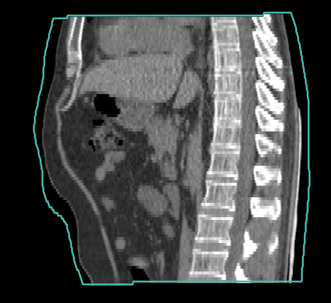
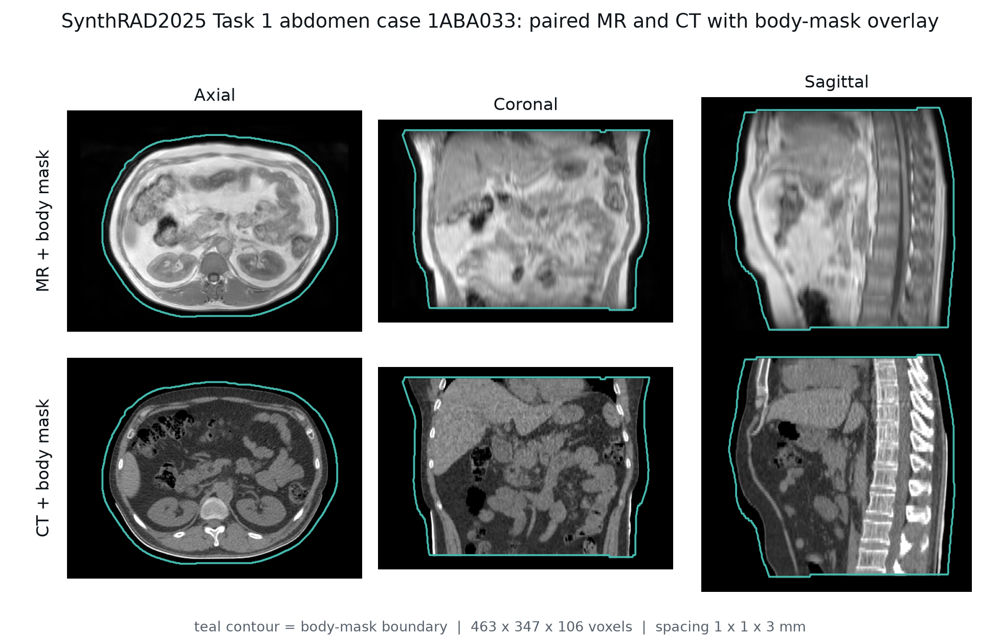
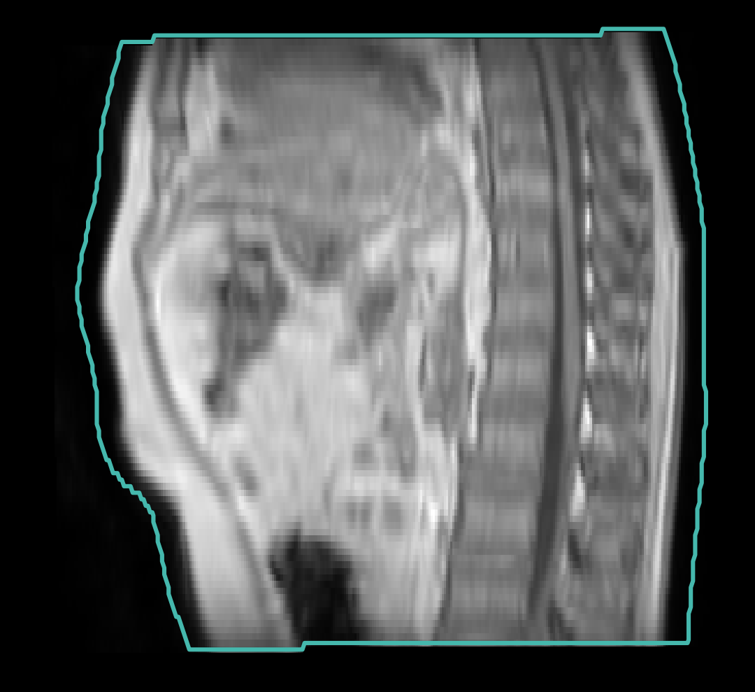
Sagittal MRI and CT from the same aligned public case. The teal contour shows the body mask.
Supervised image synthesis
fθ(xMR) = ŷCT- xMR
- input MR volume
- fθ
- network with learned parameters
- ŷCT
- predicted synthetic CT
- yCT
- aligned reference CT
Training assumption
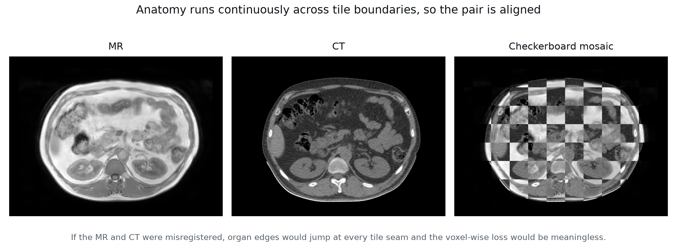
MR and CT must describe the same anatomy at the same coordinates.
Otherwise voxel-wise error mixes registration error with synthesis error.
Check your understanding
If the CT is shifted five voxels to the right, what does a voxel-wise loss measure?
Show answer
Both synthesis error and misalignment. The target at a coordinate no longer represents the same anatomy.
02
Framework
What nnsyn actually is
How nnsyn adapts nnU-Net for image synthesis
Chapter 01 defined the task: use an aligned MRI to estimate a CT value at each voxel. nnsyn organizes the complete experiment around that task. It keeps the main nnU-Net workflow for measuring the dataset, creating a plan, training on patches, saving checkpoints, and reconstructing a full volume. It adapts that workflow so the network predicts continuous image values instead of segmentation classes.
The decisive output change
| Task | Output tensor | Meaning at each voxel |
|---|---|---|
| Segmentation | [B, K, D, H, W] | K class scores |
| nnsyn synthesis | [B, 1, D, H, W] | one continuous target value |
The diagram gives the high-level view. In the code, these jobs are divided across several files. The map below shows which file answers each course question.
Read the repository by questionEach link opens the relevant source area.
nnsyn_preprocessing.pyHow do paired files become trainable arrays?
experiment_planning/How are patch, spacing, and architecture chosen?
nnUNetTrainer_nnsyn.pyWhat changes from segmentation to regression?
nnsyn_loss_map.pyWhat does the advanced loss compare?
nnsyn_predict_entrypoints.pyHow is inference wrapped and HU restored?
analysis/How are outputs evaluated and visualized?
Chapter takeaway
The dataset fingerprint determines the experiment plan, and the plan determines which network is built and how it is trained.
03
Data & plans
Data preparation and self-configuration
How nnsyn builds the training plan
Chapter 02 showed how nnsyn adapts nnU-Net. Before it can configure a network, it must organize and measure the data. For each case, one case ID links the MRI, reference CT, and mask. nnsyn then converts these files into normalized arrays and creates the training plan from the measured dataset properties.
Origin
INPUT_IMAGES/
TARGET_IMAGES/
MASKS/
LABELS/ optional
Paired medical-image files.
Raw
imagesTr/
labelsTr/
dataset.json
nnU-Net naming and identity.
Preprocessed
CASE.npy
CASE_seg.npy  # continuous CT target
CASE_mask.npy
nnUNetPlans.json
Normalized arrays and plan.
Results
fold_0/
checkpoint_*.pth
training_log*.txt
Weights and run evidence.
Self-configuration is a sequence of decisions
Fingerprint
Measure image size, spacing, orientation, and intensity.
Plan
Choose spacing, patch, batch, kernels, strides, and network depth.
Preprocess
Normalize and, when needed, resample every case consistently.
Train
Build the planned network and sample planned patches.
Verified plan · SynthRAD2025 Task 1 abdomen training data
- Spacing
- 3 × 1 × 1 mm
- Patch
- 48 × 192 × 224
- Batch
- 2 patches
- Stages
- 6 encoder levels
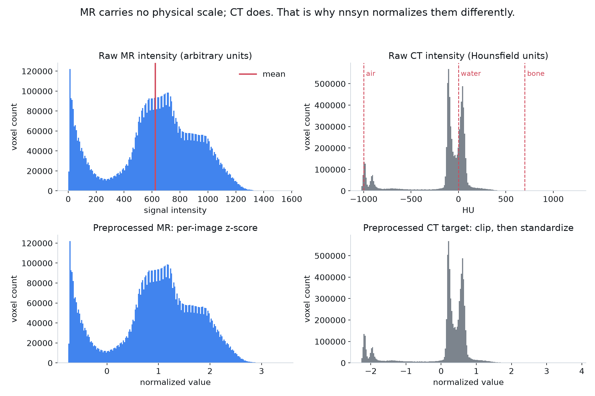
Normalization changes the numerical scale without changing the anatomy. For case 1ABA033, the complete MR volume has mean 277.33 and standard deviation 368.80. After preprocessing, the stored MR array has mean approximately 0 and standard deviation 1. This example shows the numerical transformation applied before the planned patches are sampled for training.
FOLLOW ONE CASE1ABA033 · voxel (53, 174, 231)
- Raw MRI821scanner-dependent intensity
- Full-volume z-score(821 − 277.33) / 368.80same transform used by the stored array
- Preprocessed MRI1.474network input at this voxel
Normalization inspection
Compare the intensity distributions before and after preprocessing
Check your understanding
Does z-score normalization make MRI values into Hounsfield units?
Show answer
No. It creates a stable numerical range for learning. HU restoration applies only to the predicted CT using saved CT statistics.
Reproduce this stageData and preprocessing guide
04
Architecture
Model and tensor flow
How one MRI patch becomes a CT patch
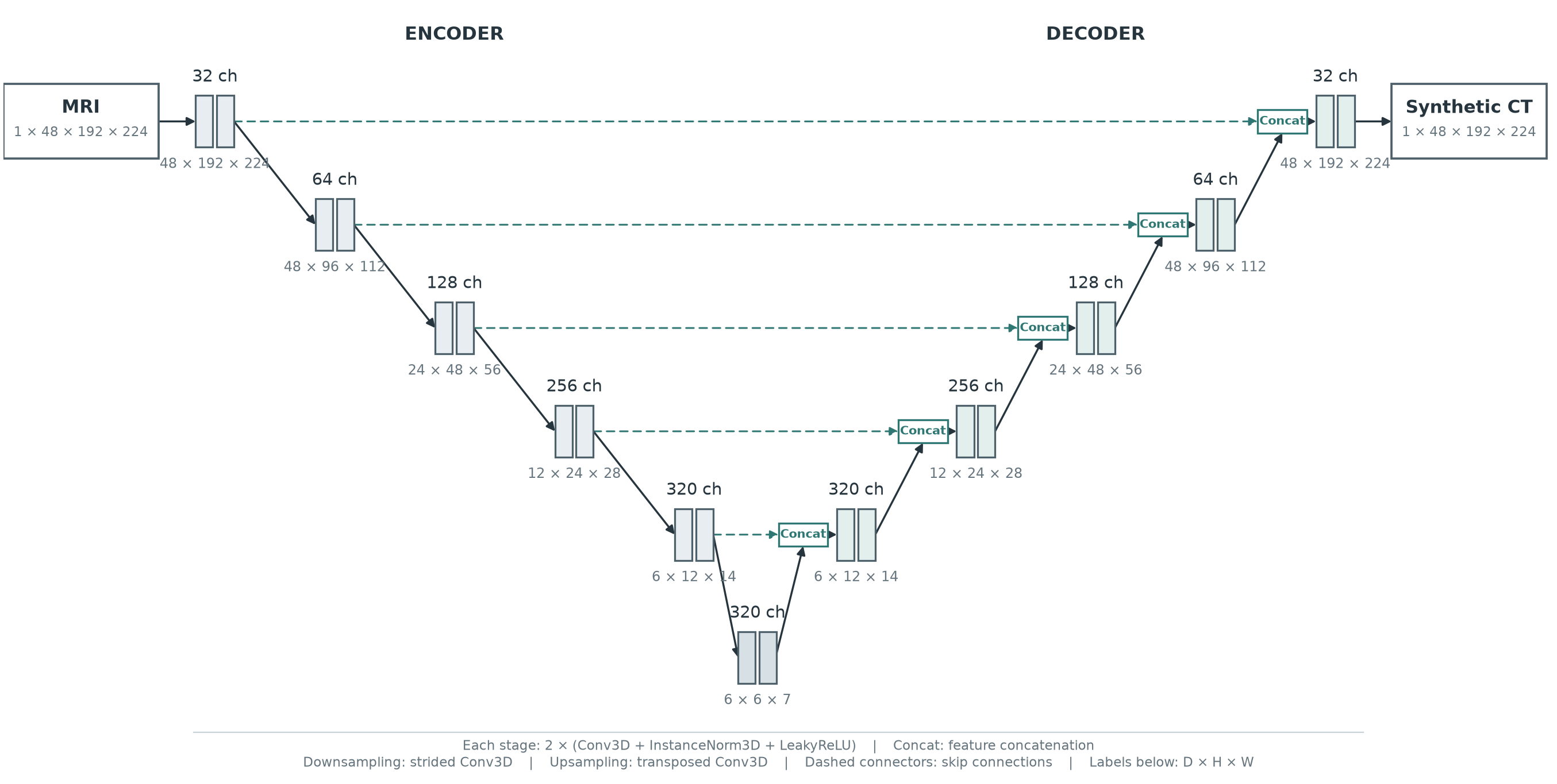
The plan from Chapter 03 fixes the patch size and network depth. The network has to do two things at once: use enough surrounding anatomy to estimate each voxel and preserve the local detail needed for accurate boundaries. The encoder builds broader context by reducing spatial resolution while increasing the number of learned feature channels.
The decoder restores the original resolution. Skip connections bring higher-resolution encoder features directly to the matching decoder stages, so the output can combine broad anatomical context with precise boundaries. This is especially important for image synthesis because every output voxel must receive a continuous value.
- Convolution
- A learned 3D filter applied throughout the volume to detect local patterns.
- Encoder
- Builds wider context while spatial dimensions shrink and feature channels grow.
- Decoder
- Turns compact contextual features back into a full-resolution prediction.
- Skip connection
- Returns spatial detail from an encoder stage to the matching decoder stage.
- Patch
- A subvolume that fits in memory; the generated plan chooses its shape.
Architecture scope
The 175-case SynthRAD2025 abdomen plan produced a six-stage PlainConvUNet with a 48 × 192 × 224 patch. nnsyn can also plan other architectures, including residual-encoder and MedNeXt variants.
05
Losses
What the model is asked to minimize
MSE, masked MSE, and MAP loss
Chapter 04 ended with a predicted CT patch. Training now needs a way to judge it. A model learns what its loss rewards: MSE compares voxel values, masking limits the comparison to the body, and MAP also compares anatomical features. The resulting loss provides the signal used to update the network.
The progression: MSE defines the numerical error → masking decides where that error can teach the network → MAP also compares anatomical features.
pi predictionti targetmi maskN all patch voxels
01
Baseline
Mean squared error
LMSE = 1N Σ (pi − ti)²
MSE compares every aligned voxel. Squaring makes large errors matter more, but it gives no special meaning to the body region or anatomical structure.
It asks: are normalized voxel values close?
02
Mask support
Masked MSE as implemented
Lmask = 1N Σ mi(pi − ti)²
For the full 1ABA033 volume, the body mask covers 44.15% of voxels. Individual training patches contain different body fractions. Multiplying by the mask makes outside-body terms zero, so those voxels do not produce gradients.
Why show this split? Masked MSE keeps the body region in the error numerator and sets the larger outside region to zero.
The repository still averages over all N patch voxels, not only Σmi foreground voxels. For one fixed patch, changing the denominator rescales the gradient without changing its direction. Across patches, however, different mask fractions change their relative scale and weighting.
repository: Σ masked error / Nalternative: Σ masked error / Σ maskIt asks: are values close in the selected body region?
03
Advanced trainer
Masked Anatomical Perception loss
predicted CTŷ
→frozen segmentorS(ŷ)
↔frozen segmentorS(y)
←reference CTy
Ltotal = (1 − w)Lperc + wLimg default w = 0.5
Limg is the repository’s masked MSE. Lperc sums L1 differences between channel-normalized feature maps from several segmentor levels. The reference features are detached; the segmentor’s weights remain fixed. Gradients from the predicted branch travel back to the synthesis network.
The two terms have equal coefficients at w = 0.5, but that does not mean their numerical magnitudes or gradients are equal. The weight controls the mixture, not a guaranteed fifty–fifty effect.
It asks: are voxel values and anatomical representations both close?
External application evidence · KoalAI validation description
| Model row | MAE ↓ | Dice ↑ | HD95 ↓ |
|---|---|---|---|
| resUnet-fold0 | 65.9640 | 0.7092 | 9.8844 |
| resUnet-MAP-fold0 | 64.5516 | 0.7436 | 8.2069 |
These are reported validation-leaderboard rows from the KoalAI algorithm description, not results from our training run and not a final-test benchmark. They illustrate why anatomical metrics may reveal changes that MAE alone does not.
See the public SASHIMI program entry for Team KoalAIReported winning recipe
ResUNet-L + MAP + five folds
KoalAI combined a large residual-encoder U-Net, Masked Anatomical Perception loss, and a five-fold ensemble. Its algorithm description reports an MAE of 62.4335 ± 23.2705 HU.
Current course reproduction
PlainConvUNet + masked MSE + one fold
Our 300-epoch baseline reached 105.0 HU mean masked MAE on its 35-case fold-0 validation set. It verifies this simpler training path, not the complete winning recipe.
Check your understanding
If w = 0.5, must perception loss and image loss contribute equally sized gradients?
Show answer
No. The coefficients are equal, but the terms can have different scales and gradient magnitudes.
06
Training
From one update to a checkpoint
One training iteration, step by step
Once the loss is defined, each training iteration follows the same sequence: load aligned patches, predict normalized CT, compute the loss, backpropagate the error, and update the weights. Validation and checkpoints record how the run progresses.
- 1
Load
MRI, target CT, and optional mask patches.
- 2
Forward
MRI patch → predicted normalized CT.
- 3
Score
Compute the selected synthesis loss.
- 4
Backward
Differentiate through the synthesis network.
- 5
Update
Clip gradient norm at 12, then change weights.
- 6
Record
Log, validate, and save checkpoints.
Repository baseline
Learning experiment
- epochs
- 1000
- iterations / epoch
- 250
- deep supervision
- off
- mirroring
- disabled by the nnsyn trainer
Course reproduction
Trained validation experiment
- cases
- 140 train / 35 validation
- epochs
- 300
- loss
- masked MSE
- device
- NVIDIA H100 80 GB
This is a trained reproduction, not the full challenge recipe.
It verifies that the repository can learn from the full public abdomen training set and produce a held-out synthetic CT. It does not reproduce every competition model, loss, fold, or ensemble.
Reproduce this stageTraining and inference guide
07
Inference
Prediction and post-processing
Reconstructing the full CT volume
Training produces a checkpoint that can predict one patch at a time. The full MRI is larger than that patch, so inference moves overlapping windows through the scan and blends their predictions into one normalized CT volume. The plan, trainer, fold, and checkpoint must match the training run so that the correct model is reconstructed.
MRI volume
→overlapping patch predictions
→normalized CT
- 1
Preprocess
Apply the training plan.
- 2
Predict
Run overlapping windows.
- 3
Blend
Combine patch predictions.
- 4
Restore HU
ŷHU = ŷ′σCT + μCT.
- 5
Apply mask
Set outside-body voxels as required.
Post-processing restores the physical CT scale
The network output is still in normalized CT space.
Saved target statistics restore Hounsfield units. The body mask then defines the valid output region and the region used for masked evaluation.
Model identity must matchdataset IDplanconfigurationtrainerfoldcheckpointchannels
Check your understanding
The raw prediction contains values close to 0. Does that mean the synthetic CT is blank?
Show answer
No. The network predicts standardized CT values, where 0 is near the training-set mean. Apply the stored CT mean and standard deviation before interpreting the image in Hounsfield units.
Reproduce this stageInference and HU-restoration guide
08
Evaluation
Numbers and images answer different questions
How synthetic CT is evaluated
Inference produces a synthetic CT in Hounsfield units. Evaluation asks how closely it matches the reference CT. A single score is not enough: metrics summarize overall error, while image panels show where those errors occur. A plausible average can still hide a failed organ boundary or a local artifact.
Read the metrics in three layers: MAE and PSNR assess CT intensities, MS-SSIM assesses visual structure, and Dice and HD95 assess anatomy derived from segmentations.
How wrong are the CT values?
MAE = (1/N) ∑ |pi − ti|Average HU difference at the evaluated voxels. MAE = 100 HU means an average error of 100 HU per voxel. Lower is better.
How small is the error relative to the image range?
PSNR = 20 log10(R / √MSE)Compares reconstruction error with the stated CT intensity range R. Higher means less error relative to that range.
Is structure preserved at different scales?
MS-SSIM = lMα ∏ cjβsjγCompares brightness, contrast, and structural patterns from fine details to larger regions. Values closer to 1 mean more similar structure.
Is the anatomy geometrically preserved?
Dice = 2|A ∩ B| / (|A| + |B|)
HD95 = P95(surface distances)
Dice measures region overlap: 1 is perfect. HD95 measures how far apart most boundaries are, usually in millimeters. Both require segmentations; Dice higher and HD95 lower are better.
Minimum visual panelMRI inputsynthetic CTreference CTabsolute error
Inspect multiple anatomical slices and include failures, not only the best-looking example.
Evaluation rule
Use the mask definition, HU restoration, metric implementation, and case split consistently. Otherwise two reported numbers may not describe the same experiment.
Reproduce this stageEvaluation and figure-generation code
09
Hands-on
Our baseline reproduction
Training nnsyn on SynthRAD2025 abdomen data
This is our 300-epoch masked-MSE baseline, not a challenge-winning result. We trained the planned 3D PlainConvUNet on 175 public SynthRAD2025 abdomen cases. Fold 0 used 140 cases for training and 35 for validation. The result below uses 1ABA101 because its error is closest to the validation median.
This experiment gives readers a complete runnable baseline and makes the remaining performance gap visible. The reported SOTA recipe is introduced in Chapter 05, but our current checkpoint should not be read as a reproduction of that recipe.
Dataset
175 paired casesSynthRAD2025 Task 1 abdomenFold 0
140 train / 35 validationall validation cases evaluatedTraining
300 epochsbest validation checkpointValidation MAE
105.0 HU mean102.0 HU median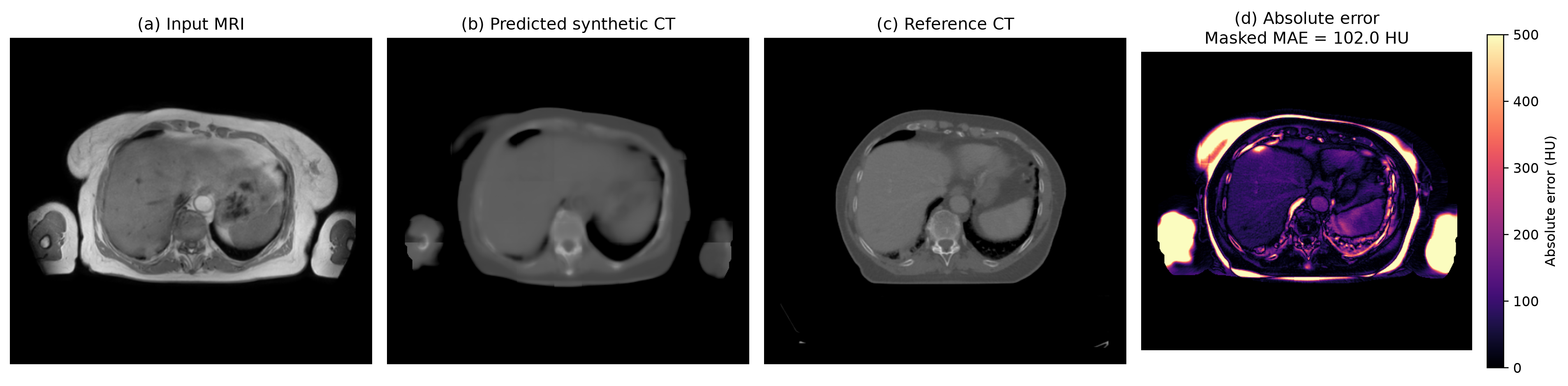
How to read this result
The model recovers the overall body shape and much of the soft-tissue intensity pattern, but its synthetic CT is visibly smoother than the reference. Bone edges and fine local details remain inaccurate. Bright regions in the error map show where the HU differences are largest.
What this result shows
- the full-data planning and preprocessing pipeline runs;
- the network learns an MRI-to-CT mapping from 140 cases;
- inference, HU restoration, masking, and evaluation complete across all 35 held-out cases.
What it does not establish
- challenge-test or external-site performance;
- five-fold or ensemble performance;
- a reproduction of MAP loss or the complete KoalAI recipe.
Validation resultsView the 35-case summary and per-case table
Portability notes from running the repositorywhat changed across Windows and Linux
Linux assumption: the trainer used SIGUSR1, which Windows does not provide. The local teaching path guarded this scheduler-specific behavior.
Inference wrapper: nnsyn_predict parses options such as worker counts and TTA control but does not forward them to the lower-level predictor. The teaching script calls that predictor directly.
Result scope: the displayed model uses the repository's masked-MSE trainer on one fold. More advanced losses, additional folds, and ensembling are separate experiments.
10
Takeaways
Close the loop
Summary and knowledge check
- 01
The core task is continuous MRI-to-CT regression, not segmentation.
- 02
nnsyn first measures the dataset, then uses those measurements to choose a training plan.
- 03
That plan fixes the spacing, patch size, batch size, and network structure used by the run.
- 04
MSE, masks, and MAP define progressively richer learning objectives.
- 05
A valid output needs matched inference, restored HU, metrics, and visual checks.
Knowledge check
Can you explain the pipeline without the diagram?
Answer first, then open each card.
1 · Why are MRI and CT not just two visual styles?
MRI intensity is acquisition-dependent; CT has calibrated HU related to X-ray attenuation. The target must be numerically meaningful.
2 · Which choices come from an nnU-Net plan?
Spacing, patch, batch size, stages, kernels, strides, and feature channels are recorded in the generated plan.
3 · Why does nnsyn write the CT target as CASE_seg.npy?
nnsyn reuses nnU-Net's internal target slot. In this synthesis pipeline, that file contains continuous normalized CT values rather than integer segmentation labels.
4 · What is unusual about the masked MSE denominator?
Masked errors are averaged over every patch voxel N, not divided by the number of foreground voxels.
5 · What does the frozen model do in MAP loss?
It extracts multiscale anatomical features from predicted and reference CT while its own weights stay fixed.
6 · Why is one held-out image not a complete performance claim?
It shows how the trained model behaves on one unseen validation case. A performance claim requires aggregate metrics over a defined validation or test cohort.
The main idea is simple: nnsyn keeps nnU-Net’s planning and training pipeline, but changes the task from classifying voxels to predicting a continuous CT value at each voxel. It also adds synthesis losses, restores predictions to HU, and evaluates them as images.
Course materials
Acknowledgements, sources, and code
Reproduce the walkthrough
Start with the verified code guideSee the tested environmentDataset and related release
SynthRAD2025 dataAEHRC SynthRAD2025 releasePrimary sources
aehrc/nnsyn repositorySynthRAD2025
Data, software, and figure provenance
| Material | How it is used here | Source and terms |
|---|---|---|
| aehrc/nnsyn | Repository studied and executed; course code is tied to commit c3ba6fd8. | Australian e-Health Research Centre; Apache License 2.0. |
| nnU-Net | Planning, preprocessing, training, and inference infrastructure inherited by nnsyn. | Isensee et al.; see the upstream paper and repository. |
| SynthRAD2025 Task 1 | Public abdomen MRI–CT data; 175 paired cases were used in our fold 0 training and validation split. Raw scans are not redistributed. | Thummerer et al.; public data and derived figures remain subject to CC BY-NC 4.0. |
| KoalAI description | External MAP-loss validation rows in Chapter 05; these are not results from our run. | Xin et al.; used here only as a cited numerical comparison. |
| Course scripts and figures | Data staging, local smoke checks, full-data training, evaluation, and visualization created for this course. | AI assistance and human verification are described below. |
AI assistance
OpenAI Codex and Anthropic Claude assisted with course organization, English revision, HTML/CSS, and supporting Python, PowerShell, Bash, and Slurm files. They were used while debugging the local Windows/CUDA setup and the Linux H100 training run, and during the final consistency review.
Human verification and responsibility
Zaiyou He ran the reported preprocessing, training, and held-out inference; inspected the logs, checkpoints, images, and numerical values; and made the final technical and editorial decisions. Codex and Claude did not generate the medical images or experimental measurements; these came from the public dataset and the reported nnsyn run. Jun Ma provided supervision and course feedback. The authors take responsibility for the final material.
References
Sources cited in this course.
- Isensee, F., Jaeger, P. F., Kohl, S. A. A., Petersen, J., and Maier-Hein, K. H. nnU-Net: a self-configuring method for deep learning-based biomedical image segmentation. Nature Methods 18, 203-211 (2021). doi:10.1038/s41592-020-01008-z
- Australian e-Health Research Centre. nnsyn: Self-configured framework for medical image synthesis. GitHub repository, commit
c3ba6fd8(accessed 31 July 2026). github.com/aehrc/nnsyn - Thummerer, A., et al. SynthRAD2025 Grand Challenge dataset: Generating synthetic CTs for radiotherapy from head to abdomen. Medical Physics 52(7), e17981 (2025). doi:10.1002/mp.17981. Dataset collection: doi:10.5281/zenodo.14918089.
- Xin, B., Sun, Z., Min, H., Belous, G., and Dowling, J. Team KoalAI: Ensembled ResUnet with Masked Anatomical Perception Loss. SynthRAD2025 algorithm description (2025).